Lesson 15. Chance is the soul of the game
You have already taught the turtle a lot. But she also has other, hidden possibilities. Can a turtle do anything on its own that will surprise you?
It turns out yes! There are turtles in the list of sensors random number sensor:
random
We often encounter random numbers: when throwing dice in a children's game, listening to a fortune teller cuckoo in the forest, or simply “guessing any number.” The random number sensor in LogoWorlds can take the value of any positive integer number from 0 to the value limit specified as a parameter.
The number itself, specified as a parameter of the random number sensor, never appears.
For example, a random sensor 20 can be any integer from 0 to 19, including 19, a random sensor 1000 can be any integer from 0 to 999, including 999.
You might be wondering where the game is - just numbers. But don’t forget that in LogoWorlds you can use numbers to set the shape of the turtle, the thickness of the writing pen, its size, color, and much more. The main thing is to choose the right limit of values. The limits of change in the basic parameters of the turtle are shown in the table.
The random number generator can be used as a parameter to any command, for example forward, right etc.
Task 24. Using the Random Number Sensor
Organize one of the games suggested below using the random number sensor and launch the turtle.
Game 1: Colorful Screen
1. Place the turtle in the center of the screen.
2. Enter commands in the Backpack and set the mode Many times:
new_color random 140 paint wait 10
Team paint performs the same actions as the Fill tool in the graphics editor.
3. Voice the plot.
Game 2: “The Cheerful Painter” 1. Modify game #1 by drawing lines on the screen into random areas with continuous boundaries:
2. Complete the instructions in the Turtle Backpack with random turns and movements:
right random 360
forward random 150
 Set instructions in the Backpack to move the turtle ( forward 60) with a 60 thick nib of random color (0-139) lowered at a slight angle ( new_course 10).
Game 4: "Hunt"
Develop a plot in which a red turtle hunts a black one. The black turtle moves along a random trajectory, and the direction of movement of the red turtle is controlled by a slider.
Questions for self-control
1. What is a random number generator?
2. What is the parameter of the random number sensor?
3. What does the value limit mean?
4. Does the number specified as a parameter ever come up?
The software of almost all computers has a built-in function for generating a sequence of pseudo-random quasi-uniformly distributed numbers. However, for statistical modeling, increased requirements are placed on random number generation. The quality of the results of such modeling directly depends on the quality of the generator of uniformly distributed random numbers, because these numbers are also sources (initial data) for obtaining other random variables with a given distribution law.
Unfortunately, ideal generators do not exist, and the list of their known properties is replenished with a list of disadvantages. This leads to the risk of using a bad generator in a computer experiment. Therefore, before conducting a computer experiment, it is necessary to either evaluate the quality of the random number generation function built into the computer, or select an appropriate random number generation algorithm.
To be used in computational physics, the generator must have the following properties:
Computational efficiency is the shortest possible calculation time for the next cycle and the amount of memory for running the generator.
Large length L random sequence of numbers. This period must include at least the set of random numbers necessary for a statistical experiment. In addition, even approaching the end of L poses a danger, which can lead to incorrect results of a statistical experiment.
The criterion for a sufficient length of a pseudorandom sequence is chosen from the following considerations. The Monte Carlo method consists of repeated calculations of the output parameters of a simulated system under the influence of input parameters that fluctuate with given distribution laws. The basis for implementing the method is the generation of random numbers with uniform distribution in the interval from which random numbers with given distribution laws are formed. Next, the probability of the simulated event is calculated as the ratio of the number of repetitions of model experiments with a successful outcome to the number of total repetitions of experiments under given initial conditions (parameters) of the model.
For a reliable, in a statistical sense, calculation of this probability, the number of repetitions of the experiment can be estimated using the formula:
Where  - function, inverse function normal distribution,
  - confidence probability of error
  Probability measurements.
Therefore, in order for the error not to go beyond the confidence interval with confidence probability, for example =0.95 it is necessary that the number of repetitions of the experiment be no less than:
 (2.2)
(2.2)
For example, for a 10% error (
=0.1) we get  , and for a 3% error (
=0.03) we already get
, and for a 3% error (
=0.03) we already get  .
.
For other initial conditions of the model, a new series of repetitions of experiments should be carried out on a different pseudo-random sequence. Therefore, either the pseudo-random sequence generation function must have a parameter that changes it (for example, R 0 ), or its length must be at least:

Where K - number of initial conditions (points on the curve determined by the Monte Carlo method), N - number of repetitions of the model experiment under given initial conditions, L - length of the pseudorandom sequence.
Then each series of N repetitions of each experiment will be carried out on its own segment of the pseudo-random sequence.
Reproducibility. As stated above, it is desirable to have a parameter that changes the generation of pseudo-random numbers. Usually this is R 0 . Therefore, it is very important that the change 0 did not spoil the quality (ie statistical parameters) of the random number generator.
Good statistical properties. This is the most important indicator quality of the random number generator. However, it cannot be assessed by any one criterion or test, because There are no necessary and sufficient criteria for the randomness of a finite sequence of numbers. The most that can be said about a pseudorandom sequence of numbers is that it “looks” random. No single statistical test is a reliable indicator of accuracy. At a minimum, it is necessary to use several tests that reflect the most important aspects of the quality of the random number generator, i.e. the degree of its approximation to an ideal generator.
Therefore, in addition to testing the generator, it is extremely important to test it using standard problems that allow independent assessment of the results by analytical or numerical methods.
It can be said that the idea of the reliability of pseudo-random numbers is created in the process of using them, with careful verification of the results whenever possible.
09.19.2017, Tue, 13:18, Moscow time , Text: Valeria Shmyrova
The Security Code company, the developer of the Continent cryptographic complex, received a patent for a biological random number sensor. This is precisely a biological sensor, since randomness is based on the user’s reaction to the image shown to him. The company assures that such technologies have not been patented in the world before.
Obtaining a patent
The Security Code company received a patent for biological random number sensor technology. According to the developers, when creating the technology, “a new approach to solving the problem of generating random numbers using a computer and a person” was used. The development is already used in a number of products, including Continent-AP, Secret Net Studio, Continent TLS and Jinn, as well as in the SCrypt cryptographic library.
As company representatives explained to CNews, work on the sensor has been going on for three years now. It consists of a scientific part, an implementation part and an experimental part. Three people are responsible for the scientific part of the company; the entire team of programmers took part in the development, and testing and experiments were carried out by the entire team, which amounts to several hundred people.
Technology capabilities
The new sensor can generate random sequences on personal devices - without the need for additional devices or hardware add-ons. It can be used in data encryption and in any area where there is a need for random binary sequences. According to the developers, it helps create encryption keys on mobile devices much faster. This property can be used to encrypt data or generate electronic signature.
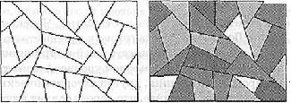
As explained Alisa Koreneva, a “Security Code” system analyst, the company’s sensor generates random sequences based on the speed and accuracy of the user’s hand response to changes in the image on the PC or tablet screen. A mouse or touchscreen is used for input. It looks like this: circles move chaotically across the screen, some of their parameters change over time. At some points in time the user reacts to changes in the image. Taking into account the peculiarities of his motor skills, this is reflected in the random mass of bits.
You can generate random number sequences based on spontaneous human reactions
Outside of cryptography, the sensor can be used to generate random numbers in computer games or to select competition winners.
Scientific novelty
As the company explained to CNews, many known methods for constructing random number sensors are based either on physical laws and phenomena, or on deterministic algorithms. Sequences can be generated using a computer - in this case, the instability of some parts of the computer and the uncertainty of hardware interference are taken as the basis for randomness.
The novelty of the Security Code technology lies in the fact that the source of randomness is a person’s reaction to a changing image that is displayed on the device’s display. That is why the name of the invention contains the word “biological”. The company reports that neither it nor Rospatent have found patented analogues of the technology in Russia or in the world. However, in general such techniques are known: for example, a sequence can be generated based on user actions such as clicks or movements of the mouse or keystrokes on the keyboard.
According to Koreneva, the development team analyzed different ways to generate random sequences. As it turned out, in many cases there are no reasonable estimates of the generation performance, or the statistical properties of the generated sequences, or both. This is due to the difficulty of justifying an already invented technology. Security Code claims that its research has produced reasonable estimates of the generation rate, was able to justify good probabilistic characteristics and statistical properties, and has estimated the entropy contributed by human actions.
Products that use technology
"Continent" is a hardware and software complex designed for data encryption. Used in the Russian public sector, for example, in the Treasury. Consists of a firewall and tools for creating a VPN. It was created by the NIP Informzashita company, and is now being developed by Security Code LLC.
Specifically, the “Continent” access server and the “Continent-AP” information cryptographic protection system are a secure module remote access using GOST algorithms, and “Continent TLS VPN” is a system for providing secure remote access to web applications also using GOST encryption algorithms.
Secret Net Studio is a comprehensive solution for protecting workstations and servers at the data, application, network, operating system and peripheral equipment, which also develops a "Security Code". Jinn-Client is designed for cryptographic information protection for creating an electronic signature and trusted visualization of documents, and Jinn-Server is a software and hardware complex for building legally significant electronic document management systems.
SCrypt cryptographic library, which also uses new sensor, was developed by the “Security Code” for more convenient application of cryptographic algorithms in various products. This is a single program code, verified for mistakes. The library supports cryptographic hashing, electronic signature, and encryption algorithms.
What does the “Security Code” do?
"Security code" - Russian company, which develops software and hardware. It was founded in 2008. The scope of the product is the protection of information systems and bringing them into compliance with international and industry standards, including the protection of confidential information, including state secrets. "Security Code" has nine licenses Federal service for Technical and Export Control (FSTEC) of Russia, the Federal Security Service (FSB) of Russia and the Ministry of Defense.
The company's staff consists of about 300 specialists; products are sold by 900 authorized partners in all regions of Russia and the CIS countries. The Security Code client base includes about 32 thousand government and commercial organizations.
Note that ideally the random number distribution density curve would look as shown in Fig. 22.3. That is, ideally, each interval contains the same number of points: N i = N/k , Where N total number points, k number of intervals, i= 1, , k .
generated theoretically by an ideal generator
It should be remembered that generating an arbitrary random number consists of two stages:
- generating a normalized random number (that is, uniformly distributed from 0 to 1);
- normalized random number conversion r i to random numbers x i, which are distributed according to the (arbitrary) distribution law required by the user or in the required interval.
Random number generators according to the method of obtaining numbers are divided into:
- physical;
- tabular;
- algorithmic.
Physical RNG
An example of a physical RNG can be: a coin (“heads” 1, “tails” 0); dice; a drum with an arrow divided into sectors with numbers; hardware noise generator (HS), which uses a noisy thermal device, for example, a transistor (Fig. 22.422.5).
| Task “Generating random numbers using a coin” | |
|
Generate a random three-digit number, uniformly distributed in the range from 0 to 1, using a coin. Precision three decimal places. |
|
The first way to solve the problem
Draw an interval from 0 to 1. Reading the numbers in sequence from left to right, split the interval in half and each time choose one of the parts of the next interval (if a 0 is rolled out, then the left one, if a 1 is rolled out, then the right one). Thus, you can get to any point in the interval, as accurately as you like. So, 1 : the interval is divided in half and , the right half is selected, the interval is narrowed: . Next number 0 : the interval is divided in half and , the left half is selected, the interval is narrowed: . Next number 0 : the interval is divided in half and , the left half is selected, the interval is narrowed: . Next number 1 : the interval is divided in half and , the right half is selected, the interval is narrowed: . According to the accuracy condition of the problem, a solution has been found: it is any number from the interval, for example, 0.625. In principle, if we take a strict approach, then the division of intervals must be continued until the left and right boundaries of the found interval COINCIDE with an accuracy of the third decimal place. That is, from the point of view of accuracy, the generated number will no longer be distinguishable from any number from the interval in which it is located.
The second way to solve the problem
|
Tabular RNG
Tabular RNGs use specially compiled tables containing verified uncorrelated, that is, in no way dependent on each other, numbers as a source of random numbers. In table Figure 22.1 shows a small fragment of such a table. By traversing the table from left to right from top to bottom, you can get random numbers evenly distributed from 0 to 1 with the required number of decimal places (in our example, we use three decimal places for each number). Since the numbers in the table do not depend on each other, the table can be traversed in different ways, for example, from top to bottom, or from right to left, or, say, you can select numbers that are in even positions.
| Table 22.1. Random numbers. Evenly random numbers distributed from 0 to 1 |
||||||||||||||||||||||||||||||||||||||||||||
| Random numbers | Evenly distributed 0 to 1 random numbers |
|||||||
| 9 | 2 | 9 | 2 | 0 | 4 | 2 | 6 | 0.929 |
| 9 | 5 | 7 | 3 | 4 | 9 | 0 | 3 | 0.204 |
| 5 | 9 | 1 | 6 | 6 | 5 | 7 | 6 | 0.269 |
The advantage of this method is that it produces truly random numbers, since the table contains verified uncorrelated numbers. Disadvantages of the method: for storage large quantity numbers require a lot of memory; There are great difficulties in generating and checking this kind of tables; repetitions when using a table no longer guarantee randomness number sequence, and therefore the reliability of the result.
There is a table containing 500 absolutely random verified numbers (taken from the book by I. G. Venetsky, V. I. Venetskaya “Basic mathematical and statistical concepts and formulas in economic analysis”).
Algorithmic RNG
The numbers generated by these RNGs are always pseudo-random (or quasi-random), that is, each subsequent number generated depends on the previous one:
r i + 1 = f(r i) .
Sequences made up of such numbers form loops, that is, there is necessarily a cycle that repeats an infinite number of times. Repeating cycles are called periods.
The advantage of these RNGs is their speed; generators require virtually no memory resources and are compact. Disadvantages: the numbers cannot be fully called random, since there is a dependence between them, as well as the presence of periods in the sequence of quasi-random numbers.
Let's consider several algorithmic methods for obtaining RNG:
- method of median squares;
- method of middle products;
- stirring method;
- linear congruent method.
Midsquare method
There is some four-digit number R 0 . This number is squared and entered into R 1. Next from R 1 takes the middle (four middle digits) new random number and writes it into R 0 . Then the procedure is repeated (see Fig. 22.6). Note that in fact, as a random number you need to take not ghij, A 0.ghij with a zero and a decimal point written on the left. This fact is reflected as in Fig. 22.6, and in subsequent similar figures.
 |
Disadvantages of the method: 1) if at some iteration the number R 0 becomes equal to zero, then the generator degenerates, so the correct choice of the initial value is important R 0 ; 2) the generator will repeat the sequence through M n steps (at best), where n number digit R 0 , M base of the number system.
For example in Fig. 22.6: if the number R 0 will be represented in the binary number system, then the sequence of pseudo-random numbers will be repeated in 2 4 = 16 steps. Note that the repetition of the sequence can occur earlier if the starting number is chosen poorly.
The method described above was proposed by John von Neumann and dates back to 1946. Since this method turned out to be unreliable, it was quickly abandoned.
Midproduct method
Number R 0 multiplied by R 1, from the result obtained R 2 the middle is extracted R 2 * (this is another random number) and multiplied by R 1. All subsequent random numbers are calculated using this scheme (see Fig. 22.7).
 |
Stirring method
The shuffle method uses operations to cyclically shift the contents of a cell left and right. The idea of the method is as follows. Let the cell store the initial number R 0 . Cyclically shifting the cell contents to the left by 1/4 of the cell length, we get a new number R 0 * . In the same way, cycling the contents of the cell R 0 to the right by 1/4 of the cell length, we get the second number R 0**. Sum of numbers R 0* and R 0** gives a new random number R 1. Next R 1 is entered in R 0, and the entire sequence of operations is repeated (see Fig. 22.8).
 |
Please note that the number resulting from the summation R 0* and R 0 ** , may not fit completely in the cell R 1. In this case, the extra digits must be discarded from the resulting number. Let us explain this in Fig. 22.8, where all cells are represented by eight binary digits. Let R 0 * = 10010001 2 = 145 10 , R 0 ** = 10100001 2 = 161 10 , Then R 0 * + R 0 ** = 100110010 2 = 306 10 . As you can see, the number 306 occupies 9 digits (in the binary number system), and the cell R 1 (same as R 0) can contain a maximum of 8 bits. Therefore, before entering the value into R 1, it is necessary to remove one “extra”, leftmost bit from the number 306, resulting in R 1 will no longer go to 306, but to 00110010 2 = 50 10 . Also note that in languages such as Pascal, “trimming” of extra bits when a cell overflows is performed automatically in accordance with the specified type of the variable.
Linear congruent method
The linear congruent method is one of the simplest and most commonly used procedures currently simulating random numbers. This method uses the mod( x, y) , which returns the remainder when the first argument is divided by the second. Each subsequent random number is calculated based on the previous random number using the following formula:
r i+ 1 = mod( k · r i + b, M) .
The sequence of random numbers obtained using this formula is called linear congruent sequence. Many authors call a linear congruent sequence when b = 0 multiplicative congruent method, and when b ≠ 0 mixed congruent method.
For a high-quality generator, it is necessary to select suitable coefficients. It is necessary that the number M was quite large, since the period cannot have more M elements. On the other hand, the division used in this method is a rather slow operation, so for a binary computer the logical choice would be M = 2 N, since in this case, finding the remainder of division is reduced inside the computer to the binary logical operation “AND”. Choosing the largest prime number is also common M, less than 2 N: in the specialized literature it is proven that in this case the low-order digits of the resulting random number r i+ 1 behave just as randomly as the older ones, which has a positive effect on the entire sequence of random numbers as a whole. As an example, one of the Mersenne numbers, equal to 2 31 1, and thus, M= 2 31 1 .
One of the requirements for linear congruent sequences is that the period length be as long as possible. The length of the period depends on the values M , k And b. The theorem we present below allows us to determine whether it is possible to achieve the period maximum length for specific values M , k And b .
Theorem. Linear congruent sequence defined by numbers M , k , b And r 0, has a period of length M if and only if:
- numbers b And M relatively simple;
- k 1 times p for every prime p, which is a divisor M ;
- k 1 is a multiple of 4, if M multiple of 4.
Finally, in conclusion, let's look at a couple of examples of using the linear congruent method to generate random numbers.
It was found that a series of pseudo-random numbers generated based on the data from example 1 would be repeated every M/4 numbers. Number q is set arbitrarily before the start of calculations, however, it should be borne in mind that the series gives the impression of being random at large k(and therefore q). The result can be improved somewhat if b odd and k= 1 + 4 · q in this case the row will be repeated every M numbers. After a long search k the researchers settled on values of 69069 and 71365.
A random number generator using the data from Example 2 will produce random, non-repeating numbers with a period of 7 million.
The multiplicative method for generating pseudorandom numbers was proposed by D. H. Lehmer in 1949.
Checking the quality of the generator
The quality of the entire system and the accuracy of the results depend on the quality of the RNG. Therefore, the random sequence generated by the RNG must satisfy a number of criteria.
The checks carried out are of two types:
- checks for uniformity of distribution;
- tests for statistical independence.
Checks for uniformity of distribution
1) The RNG should produce close to the following values of statistical parameters characteristic of a uniform random law:
2) Frequency test
A frequency test allows you to find out how many numbers fall within an interval (m r σ r ; m r + σ r) , that is (0.5 0.2887; 0.5 + 0.2887) or, ultimately, (0.2113; 0.7887). Since 0.7887 0.2113 = 0.5774, we conclude that in a good RNG, about 57.7% of all random numbers drawn should fall into this interval (see Fig. 22.9).
in case of checking it for frequency test
It is also necessary to take into account that the number of numbers falling into the interval (0; 0.5) should be approximately equal to the number of numbers falling into the interval (0.5; 1).
3) Chi-square test
The chi-square test (χ 2 test) is one of the most well-known statistical tests; it is the main method used in combination with other criteria. The chi-square test was proposed in 1900 by Karl Pearson. His remarkable work is considered as the foundation of modern mathematical statistics.
For our case, testing using the chi-square criterion will allow us to find out how much the real The RNG is close to the RNG benchmark, that is, whether it satisfies the uniform distribution requirement or not.
Frequency diagram reference The RNG is shown in Fig. 22.10. Since the distribution law of the reference RNG is uniform, then the (theoretical) probability p i getting numbers into i th interval (all these intervals k) is equal to p i = 1/k . And thus, in each of k intervals will hit smooth By p i · N numbers ( N total number of numbers generated).
A real RNG will produce numbers distributed (and not necessarily evenly!) across k intervals and each interval will contain n i numbers (in total n 1 + n 2 + + n k = N ). How can we determine how good the RNG being tested is and how close it is to the reference one? It is quite logical to consider the squared differences between the resulting number of numbers n i and "reference" p i · N . Let's add them up and the result is:
χ 2 exp. = ( n 1 p 1 · N) 2 + (n 2 p 2 · N) 2 + + ( n k p k · N) 2 .
From this formula it follows that the smaller the difference in each of the terms (and therefore the smaller the value of χ 2 exp.), the stronger the law of distribution of random numbers generated by a real RNG tends to be uniform.
In the previous expression, each of the terms is assigned the same weight (equal to 1), which in fact may not be true; therefore, for chi-square statistics, it is necessary to normalize each i th term, dividing it by p i · N :
Finally, let’s write the resulting expression more compactly and simplify it:
We obtained the chi-square test value for experimental data.
In table 22.2 are given theoretical chi-square values (χ 2 theoretical), where ν = N 1 is the number of degrees of freedom, p this is a user-specified confidence level that indicates how much the RNG should satisfy the requirements of a uniform distribution, or p is the probability that the experimental value of χ 2 exp. will be less than the tabulated (theoretical) χ 2 theor. or equal to it.
| Table 22.2. Some percentage points of the χ 2 distribution |
|||||||||||||||||||||||||||||||||||||||||||||||||||||||||||||||||||||||||||||||||||||||||||||||||||||||||||||||||||||||||||||||||||||||||||||||||||||||
| p = 1% | p = 5% | p = 25% | p = 50% | p = 75% | p = 95% | p = 99% | |
| ν = 1 | 0.00016 | 0.00393 | 0.1015 | 0.4549 | 1.323 | 3.841 | 6.635 |
| ν = 2 | 0.02010 | 0.1026 | 0.5754 | 1.386 | 2.773 | 5.991 | 9.210 |
| ν = 3 | 0.1148 | 0.3518 | 1.213 | 2.366 | 4.108 | 7.815 | 11.34 |
| ν = 4 | 0.2971 | 0.7107 | 1.923 | 3.357 | 5.385 | 9.488 | 13.28 |
| ν = 5 | 0.5543 | 1.1455 | 2.675 | 4.351 | 6.626 | 11.07 | 15.09 |
| ν = 6 | 0.8721 | 1.635 | 3.455 | 5.348 | 7.841 | 12.59 | 16.81 |
| ν = 7 | 1.239 | 2.167 | 4.255 | 6.346 | 9.037 | 14.07 | 18.48 |
| ν = 8 | 1.646 | 2.733 | 5.071 | 7.344 | 10.22 | 15.51 | 20.09 |
| ν = 9 | 2.088 | 3.325 | 5.899 | 8.343 | 11.39 | 16.92 | 21.67 |
| ν = 10 | 2.558 | 3.940 | 6.737 | 9.342 | 12.55 | 18.31 | 23.21 |
| ν = 11 | 3.053 | 4.575 | 7.584 | 10.34 | 13.70 | 19.68 | 24.72 |
| ν = 12 | 3.571 | 5.226 | 8.438 | 11.34 | 14.85 | 21.03 | 26.22 |
| ν = 15 | 5.229 | 7.261 | 11.04 | 14.34 | 18.25 | 25.00 | 30.58 |
| ν = 20 | 8.260 | 10.85 | 15.45 | 19.34 | 23.83 | 31.41 | 37.57 |
| ν = 30 | 14.95 | 18.49 | 24.48 | 29.34 | 34.80 | 43.77 | 50.89 |
| ν = 50 | 29.71 | 34.76 | 42.94 | 49.33 | 56.33 | 67.50 | 76.15 |
| ν > 30 | ν + sqrt(2 ν ) · x p+ 2/3 · x 2 p 2/3 + O(1/sqrt( ν )) | ||||||
| x p = | 2.33 | 1.64 | 0.674 | 0.00 | 0.674 | 1.64 | 2.33 |
Considered acceptable p from 10% to 90%.
If χ 2 exp. much more than χ 2 theory. (that is p is large), then the generator does not satisfy the requirement of uniform distribution, since the observed values n i go too far from theoretical p i · N and cannot be considered random. In other words, such a large confidence interval is established that the restrictions on the numbers become very loose, the requirements on the numbers become weak. In this case, a very large absolute error will be observed.
Even D. Knuth in his book “The Art of Programming” noted that having χ 2 exp. for small ones, in general, it’s also not good, although this seems, at first glance, to be wonderful from the point of view of uniformity. Indeed, take a series of numbers 0.1, 0.2, 0.3, 0.4, 0.5, 0.6, 0.7, 0.8, 0.9, 0.1, 0.2, 0.3, 0.4, 0.5, 0.6, they are ideal from the point of view of uniformity, and χ 2 exp. will be practically zero, but you are unlikely to recognize them as random.
If χ 2 exp. much less than χ 2 theory. (that is p small), then the generator does not satisfy the requirement of a random uniform distribution, since the observed values n i too close to theoretical p i · N and cannot be considered random.
But if χ 2 exp. lies in a certain range between two values of χ 2 theor. , which correspond, for example, p= 25% and p= 50%, then we can assume that the random number values generated by the sensor are completely random.
In addition, it should be borne in mind that all values p i · N must be large enough, for example more than 5 (found out empirically). Only then (with a sufficiently large statistical sample) can the experimental conditions be considered satisfactory.
So, the verification procedure is as follows.
Tests for statistical independence
1) Checking for the frequency of occurrence of numbers in the sequence
Let's look at an example. The random number 0.2463389991 consists of the digits 2463389991, and the number 0.5467766618 consists of the digits 5467766618. Connecting the sequences of digits, we have: 24633899915467766618.
It is clear that the theoretical probability p i loss i The th digit (from 0 to 9) is equal to 0.1.
2) Checking the appearance of series of identical numbers
Let us denote by n L number of series of identical digits in a row of length L. Everything needs to be checked L from 1 to m, Where m this is a user-specified number: the maximum occurring number of identical digits in a series.
In the example “24633899915467766618” 2 series of length 2 (33 and 77) were found, that is n 2 = 2 and 2 series of length 3 (999 and 666), that is n 3 = 2 .
The probability of occurrence of a series of length L is equal to: p L= 9 10 L (theoretical). That is, the probability of occurrence of a series one character long is equal to: p 1 = 0.9 (theoretical). The probability of a series of two characters appearing is: p 2 = 0.09 (theoretical). The probability of a series of three characters appearing is: p 3 = 0.009 (theoretical).
For example, the probability of occurrence of a series one character long is p L= 0.9, since there can be only one symbol out of 10, and there are 9 symbols in total (zero does not count). And the probability that two identical symbols “XX” will appear in a row is 0.1 · 0.1 · 9, that is, the probability of 0.1 that the symbol “X” will appear in the first position is multiplied by the probability of 0.1 that the same symbol will appear in the second position “X” and multiplied by the number of such combinations 9.
The frequency of occurrence of series is calculated using the chi-square formula we previously discussed using the values p L .
Note: The generator can be tested multiple times, but the tests are not complete and do not guarantee that the generator produces random numbers. For example, a generator that produces the sequence 12345678912345 will be considered ideal during tests, which is obviously not entirely true.
In conclusion, we note that the third chapter of Donald E. Knuth's book The Art of Programming (Volume 2) is entirely devoted to the study of random numbers. It studies various methods generating random numbers, statistical tests of randomness, and converting uniformly distributed random numbers to other types of random variables. More than two hundred pages are devoted to the presentation of this material.
Obtaining and converting random numbers.
There are two main ways to obtain random numbers:
1) Random numbers are generated by a special electronic attachment (random number sensor) installed on the computer. The implementation of this method requires almost no additional operations other than accessing the random number sensor.
2) Algorithmic method - based on the generation of random numbers in the machine itself using a special program. The disadvantage of this method is additional expense computer time, since in this case the machine performs the operations of the electronic set-top box itself.
A program for generating random numbers using a given distribution law can be cumbersome. Therefore, random numbers with a given distribution law are usually obtained not directly, but by transforming random numbers that have some standard distribution. Often this standard distribution is the uniform distribution (easy to obtain and easy to convert to other laws).
It is most advantageous to obtain random numbers with a uniform law using an electronic set-top box, which frees the computer from additional costs of computer time. Obtaining a purely uniform distribution on a computer is impossible due to the limited nature of the bit grid. Therefore, instead of a continuous set of numbers on the interval (0, 1), a discrete set of numbers is used 2n numbers, where n– bit depth of the machine word.
The law of distribution of such a population is called quasi-uniform . At n³20, the differences between the uniform and quasi-uniform laws become insignificant.
To obtain quasi-uniform random numbers, two methods are used:
1) generating random numbers using an electronic set-top box by modeling some random processes;
2) obtaining pseudorandom numbers using special algorithms.
To receive n-digit binary random number, the first method simulates a sequence of independent random variables z i, taking the value 0 or 1. The resulting sequence is 0 and 1, if we consider it as a fractional number, and represents a random variable of quasi-uniform distribution on the interval (0, 1). Hardware methods for obtaining these numbers differ only in the way they obtain the implementation z i.
One of the methods is based on counting the number of radioactive particles over a certain period of time Dt, if the number of particles is beyond Dt even, then z i=1 , and if odd, then z i=0 .
Another method uses the noise effect of a vacuum tube. By recording the value of noise voltage at certain points in time t i, we obtain the values of independent random variables U(t i), i.e. voltage (Volts).
Magnitude z i determined by law:
Where a– a certain value of the threshold voltage.
Magnitude a usually selected from the condition:
The disadvantage of the hardware method is that it does not allow the use of the double-run method to control the operation of the algorithm for solving any problem, since repeated runs fail to obtain the same random numbers.
Pseudorandom They call numbers generated on a computer using special programs in a recurrent manner: each random number is obtained from the previous one using special transformations.
The simplest of these transformations is the following. Let there be some n– bit binary number from the interval nО (0, 1). Let's square it, and we get 2n digit number. Let's highlight the averages n discharges. Obtained in this way n– the digit number will be the new value of the random number. We square it again, etc. This sequence is pseudorandom, because from a theoretical point of view, it is not random.
The disadvantage of recurrent algorithms is that sequences of random numbers may degenerate (for example, we will receive only a sequence of zeros or a sequence of ones, or periodicity may appear).